# init repo notebook
!git clone https://github.com/rramosp/ppdl.git > /dev/null 2> /dev/null
!mv -n ppdl/content/init.py ppdl/content/local . 2> /dev/null
!pip install -r ppdl/content/requirements.txt > /dev/null
import numpy as np
import matplotlib.pyplot as plt
import seaborn as sns
import tensorflow as tf
import tensorflow_probability as tfp
from tensorflow.keras.optimizers import Adam
from IPython.display import display, Math
plt.style.use("ggplot")
tfd = tfp.distributions
Probabilistic Linear Regression#
The linear regression is one of the simplest models in machine learning, the main goal is to compute an estimation \(\tilde{\mathbf{y}} \in \mathbb{R} ^ N\) (where \(N\) is the number of samples) of a target variable \(\mathbf{y} \in \mathbb{R} ^ N\) using some input variables \(\mathbf{X} \in \mathbb{R} ^ {N \times m}\) (where \(m\) is the number of variables) through a linear model:
Conventionally, the parameters \(\mathbf{w} \in \mathbb{R} ^ m\) are estimated through the minimization of the Mean Squared Error (MSE). However, this is equivalent to the Maximum Likelihood Estimation (MLE) of a probabilistic model. More precisely, we assume that the distribution of the label’s noise is given by a normal distribution, so it is possible to define the following model:
Where \(\epsilon \sim \mathcal{N}(\mu = 0, \sigma=E)\) and \(E\) is the noise’s magnitude or standard error. This can be summarized as the distribution of the target variables as follows:
The MLE would then consist on determining \(\mathbf{w}\) and \(E\) such that the likelihood probability is maximized, or equivalently, minimizing the negative log-likelihood.
Let’s see an example over some synthetic data:
x = tf.random.uniform(
        shape = (1000, 1),
        minval = -1,
        maxval = 1
        )
X = tf.concat([x, tf.ones_like(x)], axis=1)
display(Math(r"\mathbf{X}:"))
display(X[:5])
display(X.shape)
<tf.Tensor: shape=(5, 2), dtype=float32, numpy=
array([[-0.45172   ,  1.        ],
       [ 0.99588037,  1.        ],
       [-0.58632326,  1.        ],
       [-0.69879675,  1.        ],
       [-0.72001743,  1.        ]], dtype=float32)>
TensorShape([1000, 2])
Let’s assume the following values for \(\mathbf{w}\) and \(E\):
w_real = tf.constant([[1.0], [-1.0]])
e_real = tf.constant(0.1)
display(Math(r"\mathbf{w}:"))
display(w_real)
display(Math(r"E:"))
display(e_real)
<tf.Tensor: shape=(2, 1), dtype=float32, numpy=
array([[ 1.],
       [-1.]], dtype=float32)>
<tf.Tensor: shape=(), dtype=float32, numpy=0.1>
Using these theoretical values, We can generate the \(\mathbf{y}\) values:
y = X @ w_real + tf.random.normal(shape=(1000, 1), mean=0, stddev=e_real)
display(Math(r"\mathbf{y}:"))
display(y[:5])
display(y.shape)
<tf.Tensor: shape=(5, 1), dtype=float32, numpy=
array([[-1.6190988 ],
       [ 0.06170123],
       [-1.4506689 ],
       [-1.6691394 ],
       [-1.7425723 ]], dtype=float32)>
TensorShape([1000, 1])
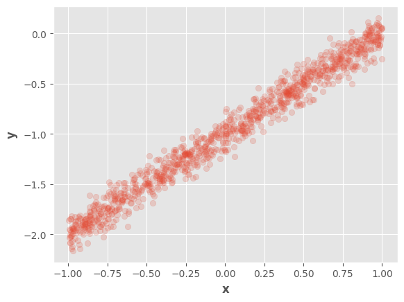
We can visualize the generated dataset:
fig, ax = plt.subplots()
ax.scatter(tf.squeeze(x), tf.squeeze(y), alpha=0.2)
ax.set_xlabel(r"$\mathbf{x}$")
ax.set_ylabel(r"$\mathbf{y}$")
fig.show()
/tmp/ipykernel_773471/3821964282.py:5: UserWarning: Matplotlib is currently using module://matplotlib_inline.backend_inline, which is a non-GUI backend, so cannot show the figure.
  fig.show()
For the estimation of these values We’ll use the automatic differentiation of tensorflow, to this end, we must define an initial set of parameters:
w = tf.Variable([[0.0], [0.0]])
e = tf.Variable(1.0)
Now, We can define a tensorflow_probability distribution:
dist = tfd.Normal(loc=X @ w, scale=e)
display(dist)
<tfp.distributions.Normal 'Normal' batch_shape=[1000, 1] event_shape=[] dtype=float32>
Let’s define the training loop:
n_iters = 100
optimizer = Adam(learning_rate=1e-2)
training_variables = [w, e]
for i in range(n_iters):
    with tf.GradientTape() as t:
        dist = tfd.Normal(loc=X @ w, scale=e)
        nll = -tf.reduce_sum(dist.log_prob(y))
        grads = t.gradient(nll, training_variables)
        optimizer.apply_gradients(zip(grads, training_variables))
We can compare the real parameters \(\mathbf{w}\) and the estimated ones \(\tilde{\mathbf{w}}\)
display(Math(r"\mathbf{w}"))
display(w_real)
display(Math(r"\tilde{\mathbf{w}}"))
display(w)
<tf.Tensor: shape=(2, 1), dtype=float32, numpy=
array([[ 1.],
       [-1.]], dtype=float32)>
<tf.Variable 'Variable:0' shape=(2, 1) dtype=float32, numpy=
array([[ 1.0003284],
       [-0.9978788]], dtype=float32)>
Also the noise’s magnitude \(E\) and the estimated one \(\tilde{E}\)
display(Math(r"E"))
display(e_real)
display(Math(r"\tilde{E}"))
display(e)
<tf.Tensor: shape=(), dtype=float32, numpy=0.1>
<tf.Variable 'Variable:0' shape=() dtype=float32, numpy=0.12940276>
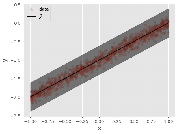
As you can see, it’s a valid probabilistic model. We can generate predictions from it:
x_test = tf.cast(
        tf.reshape(tf.linspace(start=-1, stop=1, num=100), (-1, 1)),
        tf.float32
        )
X_test = tf.concat([x_test, tf.ones_like(x_test)], axis=1)
y_pred = X_test @ w
y_pred_high = y_pred + 3 * tf.ones_like(y_pred) * e
y_pred_low = y_pred - 3 * tf.ones_like(y_pred) * e
Let’s visualize the predictions:
fig, ax = plt.subplots()
ax.scatter(tf.squeeze(x), tf.squeeze(y), alpha=0.2, label="data")
ax.plot(tf.squeeze(x_test), tf.squeeze(y_pred), label=r"$\tilde{y}$", color="k")
ax.fill_between(
    tf.squeeze(x_test),
    tf.squeeze(y_pred_low),
    tf.squeeze(y_pred_high),
    alpha=0.5, color="k"
)
ax.set_xlabel(r"$\mathbf{x}$")
ax.set_ylabel(r"$\mathbf{y}$")
ax.legend()
fig.show()
/tmp/ipykernel_773471/2646422756.py:13: UserWarning: Matplotlib is currently using module://matplotlib_inline.backend_inline, which is a non-GUI backend, so cannot show the figure.
  fig.show()